Dynamic Programming (i): Multiplying Matrices

For the last few months I’ve been interested in the concepts behind dynamic programming, however, I haven’t had time to read and learn about this topic. Now that I have started this new blog I will take the opportunity to learn about it and explain here the progress that I will be making. To share with you the code that I will be using I have created a new GH repo.

Matrix Multiplication

In this post, we will talk about how to use dynamic programming to solve the problem known as Matrix Chain Ordering Problem (MCOP),
but to be able to explain what is this problem, we need first to cover some basic concepts, starting with how to multiply matrices.

First steps

Let’s start with some notation: a matrix will be represented as a bold capital letter, ie: $\textbf{A}$; and a vector as a bold lowercase letter, ie: $\textbf{a}$. We will also use index notation, so the $i$, $j$ entry ($i$-column, $j$-row) of matrix $\textbf{A}$ is indicated by $\textbf A_{ij}$ or simplifying $A_{ij}$.

With this fixed notation, given a $m \times n$ matrix $\textbf{A}$ and a $n \times p$ matrix $\textbf{B}$

The product of $\textbf{A}$ and $\textbf{B}$ will be a $m \times p$ matrix $\textbf{C}$ - this is very important for what we are studying, so keep it in mind.

And the $i, j$ entry of $\textbf{C}$ will be

So, matrix $\textbf{C}$ will look like

From these definitions one can show that the matrix multiplication operation is associative, this means that

In other words, you can parenthesize the expression as you want and the result will always be the same.

The order matters

Now that we have covered the matrix multiplication basics let’s point out something you may have not noticed:
the order in which you multiply multiple matrices matters.

How is that possible? Didn’t we show above that the matrix multiplication is associative? How can it be that the order in which you perform the multiplications affects the result?

Well, first of all let me tell you that the matrix multiplications is still associative, and that the order only affects
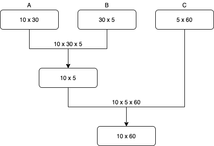
to the number of operations you will need to do. Let me show you this using a simple example. Let $\textbf{A} \in \mathbb{R}^{10 \times 30}$, $ \textbf{B} \in \mathbb{R}^{30 \times 5} $, $ \textbf{C} \in \mathbb{R}^{5 \times 60} $ and $\textbf{D} = \textbf{A}\textbf{B}\textbf{C}$. To compute $\textbf{D}$ we have two options: $\textbf{D} = (\textbf{A}\textbf{B})\textbf{C}$ (first multiply A and B, and multiply the result with C) or $\textbf{D} = \textbf{A}(\textbf{B}\textbf{C})$ (first multiply B and C, and multiply the result with A). While these two options lead to the same result the number of operations to perform is different in each case.

Before starting working out the above example, let’s notice that the number of arithmetic operations needed to compute a product of matrices $\textbf{A}\textbf{B}$ is $\mathcal{O}(nmp)$, where $\textbf{A}$ is an $n\times m$ matrix and $\textbf{B}$ is an $m\times p$ matrix.

On one hand we have the option to compute $\textbf{D}$ as $\textbf{D} = (\textbf{A}\textbf{B})\textbf{C}$. In this case, we first compute $\textbf{A}\textbf{B}$, abd we would need to perform $10 \times 30 \times 5$ multiplications. After that, we would have a $10 \times 5$ matrix and we will multipliy it with $\textbf{C}$, which will imply $10 \times 5 \times 60$ operations. In total this is 4500 operations. In the following image we have a little diagram that can help to understand what are we doing.

On the other hand, $\textbf{D} = \textbf{A}(\textbf{B}\textbf{C})$, and following the same reasoning as above (there’s below a similar diagram) we find that the number of operations in this case is 27000.

So, the first option is much more efficient. After having seen this example we are ready to formalize our problem statement.

Matrix Chain Multiplication

Problem statement

As we have shown in the last section, the multiplication order impacts the number of operations that we’ll need to perform, therefore, it makes sense to have a method to obtain the order that minimizes the number of operations. The order in which operations are carried out is determined by how the expression is parenthesized. Hance, one way to express our problem as:

How to determine the optimal parenthesization of a product of $n$ matrices.

Number of parenthesizations

It would be interesting to have an idea of how difficult this problem is, in other words, if it is possible to solve it by brute force. To answer this question we need to know how the number of possible solutions depends on $n$ for a chain of products like $A_1A_2…A_n$.

The number of possible parenthesizations for $n\geq 2$ is given by $P(n) = \sum_k P(k) P(n-k)$. The sum runs over all the possible partitions in two of the chain, and the first term of the product is the number of parenthesizations of the left partition of the chain and the second term is the number of parenthesizations of the right partition. When $n=1$ there’s only one possible parenthesization. Therefore,

And it turns out that this kind of recurrences are related with Catalan numbers, which implies that $P(n) \sim \frac{4^n}{n^{3/2}}$. Therefore, trying all the possible solutions is a bad idea.

Solutions

In this section, we will show two different solutions to this problem: a brute force one and another one smarter.

Brute Force

Even knowing that the brute force algorithm is not a feasible solution it’s interesting to implement it to be able to compare future optimizations against it. The brute force implementation is just computing all the possible partitions and the associated number of operations, and then select the partition with fewer operations. The implementation can be found here.

The main idea behind this method is implemented here:

def naive_mcm(dims: Tuple[int]) -> Tuple[int, Sequence]:
    n_matrices = len(dims) - 1
    s = [[0 for _ in range(n_matrices)] for _ in range(n_matrices)]
    def _mcm(d, i, j):
        if j <= i + 1:
            return 0
        min_cost = float('inf')
        best_partition = None
        for k in range(i + 1, j):
            cost = _mcm(d, i, k) + _mcm(d, k, j) + d[i] * d[k] * d[j]
            if cost < min_cost:
                min_cost = cost
                best_partition = k
        s[i][j - 1] = best_partition
        return min_cost
    return _mcm(dims, 0, n_matrices), s

The main point of this code is the line cost = _get_min_cost(dims_, i, k) + _get_min_cost(dims_, k, j) + dims_[i] * dims_[k] * dims_[j], where we split the problem in two: first get the minimum cost of the left partition, then we add the minimum cost of the right partition and finally add the cost of multiplying the left and right partitions.

On the other hand, we are using the matrix s to store which is the best possible partition for each possible subsequence. For a given chain of multiplications $A_1A_2…A_n$ the element $i, j$ of s store the best partition of the subsequence $A_i…A_j$. Using this matrix s we can print the best parenthesization, using the print_parenthesis method.

Memoization

In this first naive implementation, there are a lot of computations that are repeated, which slows down a lot the performance of the algorithm, and the idea behind dynamic programming is to avoid repeating all these computations. In python this can be achieved with this little piece of code:

def memoize(f):
    memo = {}
    def helper(dims, i, j):
        if (i, j) not in memo:
            memo[(i, j)] = f(dims, i, j)
        return memo[(i, j)]
    return helper

But what the heck is this? This is a python decorator. And what does it do? This decorator is an optimization technique used primarily to speed up computer programs by storing the results of expensive function calls and returning the cached result when the same inputs occur again. So by applying this decorator to the _mcm function,

@memoize
def _mcm(d, i, j):

the computations can be sped up to a thousand times. In the following section we will compare the naive and the memoized algorithms.

Brute Force vs Memoized Algorithms

In Fig. 3 we show in log-scale the time that the naive algorithm has taken to solve a problem versus the time that took to the memoized algorithm to solve the same problems. To generate each point we have solved several problems of the same size and computed the mean (dot) and the standard deviation (shaded area).

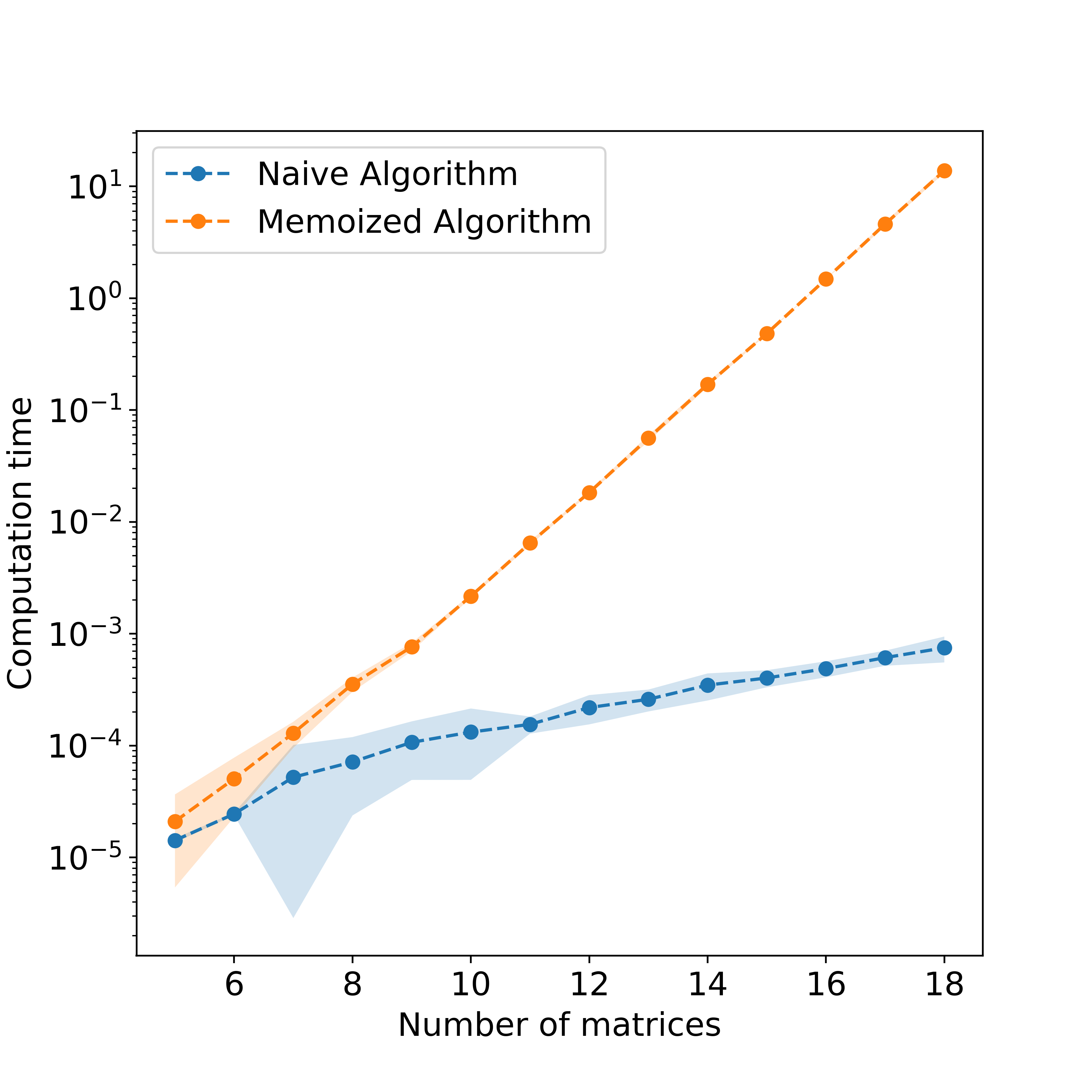
We can see that for small problems, the naive algorithm is faster than the memoized one, this could be because it takes some time to create the dictionary that stores previously solved problems. However, when the problem size increases it turns out that the memoized algorithm is much faster than the naive one. In fact, for problem sizes $\sim 18$ it’s up to $10^5$ times faster!